What does it mean to “find an effect”?#

When a model reports an effect whose credible interval excludes zero, most analysts exhale. The intervention worked. Ship the slide deck.

But excluding zero is a statement about parameter uncertainty — the noise inside the model. It tells you that, conditional on the model being correct, the data are unlikely to have been generated by a zero effect. That conditional clause does most of the heavy lifting, and it is almost never true.

Every quasi-experimental method rests on identifying assumptions: parallel trends, no anticipation, no interference. When those assumptions crack, and they always crack a little, the model’s counterfactual drifts from truth. Bugaev & Trujillo (2026) call this gap the structural error: the systematic deviation between what the model promises and what reality delivers. Standard credible intervals are blind to it.

Gallea puts the epistemological point sharply:

“We cannot prove causality with a simple test […] the most important assumption, called the unconfoundedness assumption, is usually not testable. We can only assess how plausible the assumption is.” — Gallea (2026)

So we cannot prove that a policy worked. What we can do is behave like causal detectives, accumulate evidence from multiple angles, stress-test our estimator, and ask whether the story holds together. Each piece of evidence is small. The argument is the pile.

This notebook demonstrates the full detective workflow on a real policy question, using CausalPy.

The case: the UK’s 2013 Carbon Price Floor#

In April 2013, the UK introduced the Carbon Price Floor (CPF), a top-up tax on carbon emissions from electricity generation. The EU’s Emissions Trading System was supposed to make dirty power expensive, but the carbon price had collapsed to around EUR 5/tonne. The CPF set a floor well above that, deliberately designed to make coal power unprofitable relative to gas and renewables.

The causal question: Did the Carbon Price Floor reduce coal Co2 ~ emissions in the UK?

We will answer this in four steps, each one small and honest:

Step	Question	What we learn
1. Estimate	Did coal Co2 drop after 2013?	The size and direction of the change
2. Calibrate	How often does this model hallucinate effects?	Whether we should trust the estimator at all
3. Trace the mechanism	If coal died, where did the energy go?	Whether the substitution story is consistent
4. Check the boundary	Did total Co2 or energy demand change?	Whether something else explains the result

No single step is conclusive. Together, they build a case.

Setup#

import warnings

import matplotlib.pyplot as plt
import matplotlib.patches as mpatches
import numpy as np
import pandas as pd

import causalpy as cp

warnings.filterwarnings("ignore")

/opt/anaconda3/envs/CausalPy/lib/python3.13/site-packages/pymc_extras/model/marginal/graph_analysis.py:10: FutureWarning: `pytensor.graph.basic.io_toposort` was moved to `pytensor.graph.traversal.io_toposort`. Calling it from the old location will fail in a future release.
  from pytensor.graph.basic import io_toposort

The data#

We combine two open datasets from Our World in Data: annual Co2 emissions and energy generation by source. We focus on the UK from 1990 to 2018 — 23 years before the policy and 5 after.

CO2_URL = "https://nyc3.digitaloceanspaces.com/owid-public/data/co2/owid-co2-data.csv"
ENERGY_URL = (
    "https://nyc3.digitaloceanspaces.com/owid-public/data/energy/owid-energy-data.csv"
)

MIN_YEAR = 1990
MAX_YEAR = 2018

# --- CO2 data ---
df_co2 = pd.read_csv(CO2_URL)
df_co2 = df_co2[
    (df_co2["country"] == "United Kingdom")
    & (df_co2["year"] >= MIN_YEAR)
    & (df_co2["year"] <= MAX_YEAR)
].copy()

# --- Energy data ---
df_energy = pd.read_csv(ENERGY_URL)
df_energy = df_energy[
    (df_energy["country"] == "United Kingdom")
    & (df_energy["year"] >= MIN_YEAR)
    & (df_energy["year"] <= MAX_YEAR)
][["year", "coal_electricity"]].copy()

# Merge on year
df_uk = df_co2.merge(df_energy, on="year", how="left")

# ITS needs a DatetimeIndex
df_uk["date"] = pd.to_datetime(df_uk["year"], format="%Y")
df_uk = df_uk.set_index("date").sort_index()

treatment_time = pd.to_datetime("2013-01-01")

print(f"UK observations: {len(df_uk)}")
print(f"Years: {df_uk['year'].min()} – {df_uk['year'].max()}")
print(f"Treatment: {treatment_time.year}")
print(f"Pre-treatment: {len(df_uk.loc[: treatment_time - pd.Timedelta(days=1)])} years")
print(f"Post-treatment: {len(df_uk.loc[treatment_time:])} years")
df_uk[["year", "co2", "coal_co2", "coal_electricity", "energy_per_gdp"]].head(10)

UK observations: 29
Years: 1990 – 2018
Treatment: 2013
Pre-treatment: 23 years
Post-treatment: 6 years

	year	co2	coal_co2	coal_electricity	energy_per_capita
date
1990-01-01	1990	601.945	252.690	206.44	43845.023
1991-01-01	1991	609.413	253.623	211.46	44652.039
1992-01-01	1992	593.846	237.747	193.64	44259.449
1993-01-01	1993	579.613	207.686	171.25	44663.285
1994-01-01	1994	574.017	195.376	161.34	44021.512
1995-01-01	1995	566.159	181.699	155.21	44062.301
1996-01-01	1996	586.761	173.072	147.27	46080.582
1997-01-01	1997	562.708	154.729	121.97	45150.043
1998-01-01	1998	568.544	154.088	122.97	45374.645
1999-01-01	1999	561.650	138.313	106.18	45010.832

Looking at the data#

Before fitting anything, look. Patterns you can see with your eyes are more robust than patterns that require a model to reveal.

fig, axes = plt.subplots(2, 2, figsize=(14, 8))

# CO2
ax = axes[0, 0]
ax.plot(df_uk.index, df_uk["co2"], "o-", color="#E24A33", lw=1.5, ms=3)
ax.axvline(treatment_time, ls="--", color="k", alpha=0.5)
ax.set_ylabel("Million tonnes CO₂")
ax.set_title("CO₂ emissions")

# Coal CO2
ax = axes[0, 1]
ax.plot(df_uk.index, df_uk["coal_co2"], "d-", color="#988ED5", lw=1.5, ms=3)
ax.axvline(treatment_time, ls="--", color="k", alpha=0.5)
ax.set_ylabel("Million tonnes CO₂")
ax.set_title("Coal CO₂ emissions")

# Coal electricity
ax = axes[1, 0]
ax.plot(df_uk.index, df_uk["coal_electricity"], "s-", color="#348ABD", lw=1.5, ms=3)
ax.axvline(treatment_time, ls="--", color="k", alpha=0.5)
ax.set_ylabel("TWh")
ax.set_title("Coal electricity generation")

# Energy per capita
ax = axes[1, 1]
ax.plot(df_uk.index, df_uk["energy_per_capita"], "^-", color="#8EBA42", lw=1.5, ms=3)
ax.axvline(treatment_time, ls="--", color="k", alpha=0.5)
ax.set_ylabel("kWh per person")
ax.set_title("Energy consumption per capita")

for ax in axes.flat:
    ax.tick_params(axis="x", rotation=45)

fig.suptitle(
    "United Kingdom, 1990–2018  (dashed line = Carbon Price Floor, 2013)",
    fontsize=10,
    y=1.00,
)
fig.tight_layout()
plt.show()

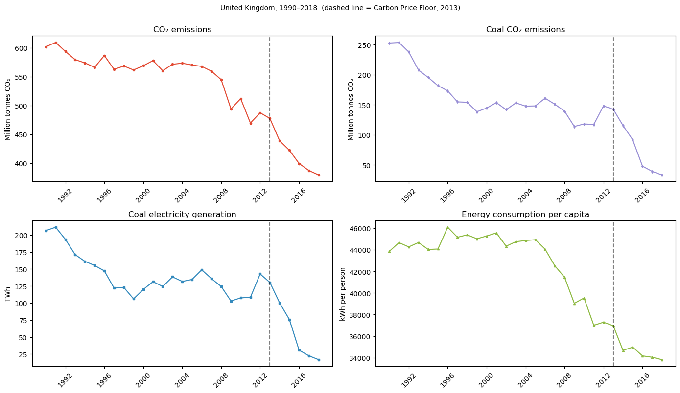
../_images/32a10de1852ea0709e95ea6e1fb6e1d3df0cfaf71cc8e0d9c3b5e3d6e8aafce7.png

Four series, one dashed line. Coal Co2 ~ and coal electricity show a visible break after 2013. Total Co2 declines more gently. Energy per capita drifts down throughout, with no obvious discontinuity.

These are eyeball impressions. Now, we need a model.

Estimate the effect on coal Co2#

Why coal Co2?#

The Carbon Price Floor was a tax on electricity generation from fossilfuels. Its direct, first-order target was coal. If we want the sharpest test of whether the policy worked, we should measure the outcome closest to the mechanism: coal Co2 emissions.

Total Co2 is tempting because it is the ultimate goal, but it mixes the policy’s direct effect with dozens of other forces (transport, industry, heating). Starting with the sharpest outcome gives us the strongest signal-to-noise ratio.

The model#

We use CausalPy’s BayesianBasisExpansionTimeSeries, a flexible Bayesian model that captures nonlinear trends via basis functions and changepoints. It fits the pre-treatment data and projects forward; the gap between projection and reality is the estimated effect.

sampler_kwargs = {
    "target_accept": 0.94,
}


def its_model():
    """Fresh BayesianBasisExpansionTimeSeries model (single-use)."""
    return cp.pymc_models.BayesianBasisExpansionTimeSeries(
        n_order=4,
        n_changepoints_trend=18,
        prior_sigma=0.05,
        sample_kwargs=sampler_kwargs,
    )

result_coal_co2 = cp.InterruptedTimeSeries(
    data=df_uk[["coal_co2"]],
    treatment_time=treatment_time,
    formula="coal_co2 ~ 1",
    model=its_model(),
)

Initializing NUTS using jitter+adapt_diag...
Multiprocess sampling (4 chains in 4 jobs)
NUTS: [fourier_beta, delta, beta, sigma]

Sampling 4 chains for 1_000 tune and 1_000 draw iterations (4_000 + 4_000 draws total) took 70 seconds.
Chain 0 reached the maximum tree depth. Increase `max_treedepth`, increase `target_accept` or reparameterize.
Chain 1 reached the maximum tree depth. Increase `max_treedepth`, increase `target_accept` or reparameterize.
Chain 2 reached the maximum tree depth. Increase `max_treedepth`, increase `target_accept` or reparameterize.
Chain 3 reached the maximum tree depth. Increase `max_treedepth`, increase `target_accept` or reparameterize.
Sampling: [beta, delta, fourier_beta, sigma, y_hat]
Sampling: [y_hat]

Sampling: [y_hat]
Sampling: [y_hat]
Sampling: [y_hat]

fig, axes = result_coal_co2.plot(show=False)
axes[0].set_title("ITS (State-Space) — UK Coal CO₂ Emissions")
plt.tight_layout()
plt.show()

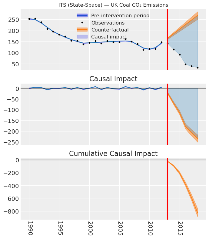
../_images/cf261dfd300857f400d37eba3b075dc75697d1ab25a0345b7dcb8029622b79f4.png

The model reports a large negative effect. Coal Co2 fell far below what the pre-treatment trend would predict. The credible interval excludes zero comfortably.

But recall our opening point. An interval that excludes zero tells us about parameter noise, not about whether the model’s assumptions hold. Before we celebrate, we need to ask: how often does this estimator hallucinate effects of this size when nothing happened?

How often does the model lie?#

The structural error problem#

Standard Bayesian credible intervals capture two kinds of uncertainty:

Aleatoric: irreducible noise in the data.
Epistemic (parameter): uncertainty about model parameters that shrinks with more data.

But there is a third kind: structural uncertainty. When the model’s identifying assumptions are violated, and they always are, at least a little. The counterfactual prediction drifts from truth. The model doesn’t know it is wrong. It reports a tight interval around a biased estimate.

Placebo-in-Time: calibrating the thermometer#

The idea is simple. Before you use the model on the real treatment date, run it on periods where you know nothing happened:

Shift the treatment date backward into the pre-treatment period.
Re-fit the model at the fake date.
Repeat for several placebo windows.
Pool the results into a hierarchical null model.

Each placebo fit asks: “How big an ‘effect’ does the model find when the true effect is zero?” The distribution of those false alarms is the null predictive distribution, what structural noise looks like for this estimator on this data.

The real effect is meaningful only if it is clearly outside this distribution. Not outside zero, instead outside the range of normal model failures.

Running the calibration with CausalPy#

CausalPy’s Pipeline composes the estimation and the sensitivity check into a single reproducible call.

result_pit = cp.Pipeline(
    data=df_uk[["coal_co2"]],
    steps=[
        cp.EstimateEffect(
            method=cp.InterruptedTimeSeries,
            treatment_time=treatment_time,
            formula="coal_co2 ~ 1",
            model=its_model(),
        ),
        cp.SensitivityAnalysis(
            checks=[
                cp.checks.PlaceboInTime(
                    n_folds=3, selection_method="random", min_gap=2
                ),
            ]
        ),
    ],
).run()

Initializing NUTS using jitter+adapt_diag...
Multiprocess sampling (4 chains in 4 jobs)
NUTS: [fourier_beta, delta, beta, sigma]

Sampling 4 chains for 1_000 tune and 1_000 draw iterations (4_000 + 4_000 draws total) took 69 seconds.
Chain 0 reached the maximum tree depth. Increase `max_treedepth`, increase `target_accept` or reparameterize.
Chain 1 reached the maximum tree depth. Increase `max_treedepth`, increase `target_accept` or reparameterize.
Chain 2 reached the maximum tree depth. Increase `max_treedepth`, increase `target_accept` or reparameterize.
Chain 3 reached the maximum tree depth. Increase `max_treedepth`, increase `target_accept` or reparameterize.
Sampling: [beta, delta, fourier_beta, sigma, y_hat]
Sampling: [y_hat]

Sampling: [y_hat]
Sampling: [y_hat]
Sampling: [y_hat]
Initializing NUTS using jitter+adapt_diag...
Multiprocess sampling (4 chains in 4 jobs)
NUTS: [fourier_beta, delta, beta, sigma]

Sampling 4 chains for 1_000 tune and 1_000 draw iterations (4_000 + 4_000 draws total) took 68 seconds.
Chain 0 reached the maximum tree depth. Increase `max_treedepth`, increase `target_accept` or reparameterize.
Chain 1 reached the maximum tree depth. Increase `max_treedepth`, increase `target_accept` or reparameterize.
Chain 2 reached the maximum tree depth. Increase `max_treedepth`, increase `target_accept` or reparameterize.
Chain 3 reached the maximum tree depth. Increase `max_treedepth`, increase `target_accept` or reparameterize.
Sampling: [beta, delta, fourier_beta, sigma, y_hat]
Sampling: [y_hat]

Sampling: [y_hat]
Sampling: [y_hat]
Sampling: [y_hat]
Initializing NUTS using jitter+adapt_diag...
Multiprocess sampling (4 chains in 4 jobs)
NUTS: [fourier_beta, delta, beta, sigma]

Sampling 4 chains for 1_000 tune and 1_000 draw iterations (4_000 + 4_000 draws total) took 67 seconds.
Chain 0 reached the maximum tree depth. Increase `max_treedepth`, increase `target_accept` or reparameterize.
Chain 1 reached the maximum tree depth. Increase `max_treedepth`, increase `target_accept` or reparameterize.
Chain 2 reached the maximum tree depth. Increase `max_treedepth`, increase `target_accept` or reparameterize.
Chain 3 reached the maximum tree depth. Increase `max_treedepth`, increase `target_accept` or reparameterize.
Sampling: [beta, delta, fourier_beta, sigma, y_hat]
Sampling: [y_hat]

Sampling: [y_hat]
Sampling: [y_hat]
Sampling: [y_hat]
Initializing NUTS using jitter+adapt_diag...
Multiprocess sampling (4 chains in 4 jobs)
NUTS: [fourier_beta, delta, beta, sigma]

Sampling 4 chains for 1_000 tune and 1_000 draw iterations (4_000 + 4_000 draws total) took 69 seconds.
Chain 0 reached the maximum tree depth. Increase `max_treedepth`, increase `target_accept` or reparameterize.
Chain 1 reached the maximum tree depth. Increase `max_treedepth`, increase `target_accept` or reparameterize.
Chain 2 reached the maximum tree depth. Increase `max_treedepth`, increase `target_accept` or reparameterize.
Chain 3 reached the maximum tree depth. Increase `max_treedepth`, increase `target_accept` or reparameterize.
Sampling: [beta, delta, fourier_beta, sigma, y_hat]
Sampling: [y_hat]

Sampling: [y_hat]
Sampling: [y_hat]
Sampling: [y_hat]
Initializing NUTS using jitter+adapt_diag...
Multiprocess sampling (4 chains in 4 jobs)
NUTS: [mu_status_quo, tau_status_quo, fold_z]

Sampling 4 chains for 1_000 tune and 1_000 draw iterations (4_000 + 4_000 draws total) took 4 seconds.
Sampling: [theta_new]

pit_check = result_pit.sensitivity_results[0]
print(pit_check.text)

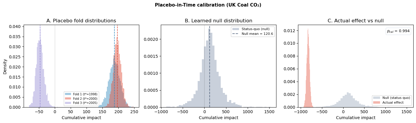
Placebo-in-time analysis: 3 of 3 folds completed.
Hierarchical status-quo model: mu=109.52, tau=188.24.
Actual cumulative impact: -826.78. P(actual outside null) = 0.994.
SUPPORTED — actual effect is outside the null distribution.
Fold 1: pseudo treatment at 1998-01-01 00:00:00 — mean=187.63, sd=17.04
Fold 2: pseudo treatment at 2000-01-01 00:00:00 — mean=196.52, sd=12.25
Fold 3: pseudo treatment at 2005-01-01 00:00:00 — mean=-46.45, sd=11.89

Visualising what the estimator sees when nothing happens#

def plot_placebo_calibration(
    pit_check, original_result, title="Placebo-in-Time calibration"
):
    """
    Plots the three-panel diagnostic for a PlaceboInTime check.

    Parameters:
    -----------
    pit_check : cp.checks.PlaceboInTime
        The completed placebo check object.
    original_result : cp.InterruptedTimeSeries (or similar)
        The original fitted causal model (needed to extract the actual post-treatment impact).
    title : str
        The main title for the figure.
    """
    fold_results = pit_check.metadata["fold_results"]
    has_null = "null_samples" in pit_check.metadata

    if not has_null:
        print("Not enough folds completed to build a null model.")
        print(f"Completed folds: {len(fold_results)}")
        if fold_results:
            for fr in fold_results:
                print(f"  Fold {fr.fold}: mean={fr.fold_mean:.2f}, sd={fr.fold_sd:.2f}")
        return

    null_samples = pit_check.metadata["null_samples"]
    _ = pit_check.metadata["actual_cumulative_mean"]

    # Fold-level cumulative impact samples
    fold_samples = [fr.cumulative_impact_samples.values.ravel() for fr in fold_results]

    FOLD_COLORS = ["#348ABD", "#E24A33", "#988ED5", "#8EBA42", "#FFB347"]
    fig, axes = plt.subplots(1, 3, figsize=(14, 4))

    # Panel A: fold distributions
    ax = axes[0]
    for i, (fr, s) in enumerate(zip(fold_results, fold_samples)):
        c = FOLD_COLORS[i % len(FOLD_COLORS)]
        # Handle datetime vs integer pseudo_treatment_time formatting
        t_star = fr.pseudo_treatment_time
        t_label = f"{t_star:%Y}" if hasattr(t_star, "strftime") else f"{t_star}"

        ax.hist(
            s,
            bins=40,
            alpha=0.45,
            color=c,
            density=True,
            label=f"Fold {fr.fold} (t*={t_label})",
        )
        ax.axvline(fr.fold_mean, color=c, ls="--", lw=1.2)
    ax.axvline(0, color="k", ls=":", lw=0.8, alpha=0.5)
    ax.set_xlabel("Cumulative impact")
    ax.set_ylabel("Density")
    ax.set_title("A. Placebo fold distributions")
    ax.legend(fontsize=7)

    # Panel B: null distribution
    ax = axes[1]
    ax.hist(
        null_samples,
        bins=50,
        alpha=0.5,
        color="#94a3b8",
        density=True,
        label="Status-quo (null)",
    )
    ax.axvline(0, color="k", ls=":", lw=0.8, alpha=0.5)
    ax.axvline(
        np.mean(null_samples),
        color="#64748b",
        ls="--",
        lw=1.5,
        label=f"Null mean = {np.mean(null_samples):.1f}",
    )
    ax.set_xlabel("Cumulative impact")
    ax.set_title("B. Learned null distribution")
    ax.legend(fontsize=8)

    # Panel C: null vs actual (overlapping distributions)
    ax = axes[2]
    # Sum of pointwise impact over post-treatment period (matches null construction)
    actual_samples = (
        original_result.post_impact.sum("obs_ind")
        .stack(sample=("chain", "draw"))
        .values.ravel()
    )
    ax.hist(
        null_samples,
        bins=50,
        alpha=0.4,
        color="#94a3b8",
        density=True,
        label="Null (status quo)",
    )
    ax.hist(
        actual_samples,
        bins=50,
        alpha=0.4,
        color="#E24A33",
        density=True,
        label="Actual effect",
    )

    p_cal = pit_check.metadata["p_effect_outside_null"]
    ax.text(
        0.97,
        0.95,
        f"$p_{{cal}}$ = {p_cal:.3f}",
        transform=ax.transAxes,
        fontsize=9,
        va="top",
        ha="right",
        bbox=dict(boxstyle="round,pad=0.3", facecolor="white", edgecolor="#e2e8f0"),
    )

    ax.set_xlabel("Cumulative impact")
    ax.set_title("C. Actual effect vs null")
    ax.legend(fontsize=8)

    fig.suptitle(title, fontsize=11, fontweight="bold", y=1.02)
    fig.tight_layout()
    plt.show()

The coal Co2 effect is massive and clearly separated from the null. Good. But even a well-calibrated thermometer can still be pointed at the wrong thing. We need to check the mechanism.

plot_placebo_calibration(
    pit_check=pit_check,
    original_result=result_pit.experiment,
    title="Placebo-in-Time calibration (UK Coal CO₂)",
)

../_images/1a656fb0b9c567cfc51f0229ac104cb5f295fea61c1b0f6f79c9f8afaf54ab80.png

Falsification: Where did the energy go?#

The detective’s logic#

Gallea (2026) tells a fascinating story about Walker Hanlon, who studied the effect of London fog on mortality. Death rates spiked during fog weeks. His hypothesis: fog traps pollution, increasing respiratory disease. But a good detective asks: could the deaths be from traffic accidents (poor visibility)? Or crime (fog as cover)?. Pneumonia spiked. Accidents and crime didn’t. Only the outcome that should respond to pollution actually did.

We apply the same logic. The Carbon Price Floor taxes carbon from electricity generation. If it works, the energy system should reorganise: coal dies, but energy demand doesn’t vanish. The electrons have to come from somewhere. The most likely substitute in 2013 was natural gas, cheaper than coal once the carbon floor bit, and already available at scale.

If gas Co2 rose after 2013, that is evidence of substitution. It means the policy didn’t reduce energy production; it redirected it. And that makes the coal Co2 decline much harder to attribute to a recession or data artefact.

Did gas Co2 rise?#

result_pit_gas = cp.Pipeline(
    data=df_uk[["gas_co2"]],
    steps=[
        cp.EstimateEffect(
            method=cp.InterruptedTimeSeries,
            treatment_time=treatment_time,
            formula="gas_co2 ~ 1",
            model=its_model(),
        ),
        cp.SensitivityAnalysis(
            checks=[
                cp.checks.PlaceboInTime(
                    n_folds=3, selection_method="random", min_gap=2
                ),
            ]
        ),
    ],
).run()

Initializing NUTS using jitter+adapt_diag...
Multiprocess sampling (4 chains in 4 jobs)
NUTS: [fourier_beta, delta, beta, sigma]

Sampling 4 chains for 1_000 tune and 1_000 draw iterations (4_000 + 4_000 draws total) took 54 seconds.
Sampling: [beta, delta, fourier_beta, sigma, y_hat]
Sampling: [y_hat]

Sampling: [y_hat]
Sampling: [y_hat]
Sampling: [y_hat]
Initializing NUTS using jitter+adapt_diag...
Multiprocess sampling (4 chains in 4 jobs)
NUTS: [fourier_beta, delta, beta, sigma]

Sampling 4 chains for 1_000 tune and 1_000 draw iterations (4_000 + 4_000 draws total) took 28 seconds.
Sampling: [beta, delta, fourier_beta, sigma, y_hat]
Sampling: [y_hat]

Sampling: [y_hat]
Sampling: [y_hat]
Sampling: [y_hat]
Initializing NUTS using jitter+adapt_diag...
Multiprocess sampling (4 chains in 4 jobs)
NUTS: [fourier_beta, delta, beta, sigma]

Sampling 4 chains for 1_000 tune and 1_000 draw iterations (4_000 + 4_000 draws total) took 34 seconds.
Sampling: [beta, delta, fourier_beta, sigma, y_hat]
Sampling: [y_hat]

Sampling: [y_hat]
Sampling: [y_hat]
Sampling: [y_hat]
Initializing NUTS using jitter+adapt_diag...
Multiprocess sampling (4 chains in 4 jobs)
NUTS: [fourier_beta, delta, beta, sigma]

Sampling 4 chains for 1_000 tune and 1_000 draw iterations (4_000 + 4_000 draws total) took 39 seconds.
Sampling: [beta, delta, fourier_beta, sigma, y_hat]
Sampling: [y_hat]

Sampling: [y_hat]
Sampling: [y_hat]
Sampling: [y_hat]
Initializing NUTS using jitter+adapt_diag...
Multiprocess sampling (4 chains in 4 jobs)
NUTS: [mu_status_quo, tau_status_quo, fold_z]

Sampling 4 chains for 1_000 tune and 1_000 draw iterations (4_000 + 4_000 draws total) took 2 seconds.
The rhat statistic is larger than 1.01 for some parameters. This indicates problems during sampling. See https://arxiv.org/abs/1903.08008 for details
Sampling: [theta_new]

pit_check_gas = result_pit_gas.sensitivity_results[0]
print(pit_check_gas.text)

Placebo-in-time analysis: 3 of 3 folds completed.
Hierarchical status-quo model: mu=-91.89, tau=124.09.
Actual cumulative impact: 275.27. P(actual outside null) = 0.890.
NOT SUPPORTED — actual effect is within the null distribution.
Fold 1: pseudo treatment at 1997-01-01 00:00:00 — mean=-193.59, sd=15.14
Fold 2: pseudo treatment at 2003-01-01 00:00:00 — mean=-6.69, sd=13.19
Fold 3: pseudo treatment at 2005-01-01 00:00:00 — mean=-79.33, sd=11.74

plot_placebo_calibration(
    pit_check=pit_check_gas,
    original_result=result_pit_gas.experiment,
    title="Placebo-in-Time calibration (UK Gas CO₂)",
)

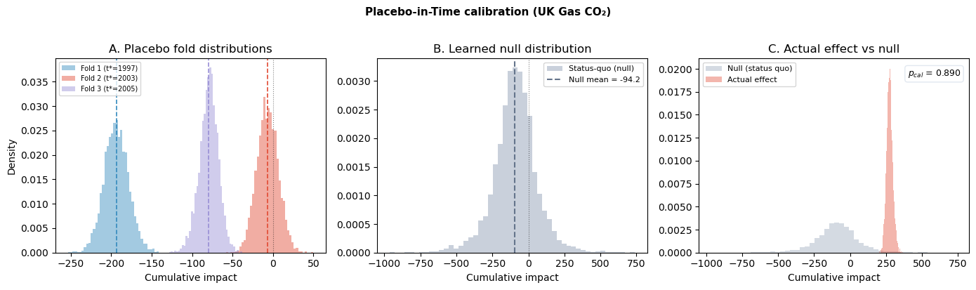
../_images/d97fdbd86e48903e31f1dfda69868f1d1260c14ade57ebec824720d2e32e1e94.png

As we thought, looks like the energy system didn’t shrink, it reorganised. Coal’s share was absorbed by gas-fired generation, exactly as the policy intended. This is the substitution channel in action.

But notice the implication: if coal Co2 went down and gas Co2 went up, the net effect on total Co2 may be smaller than either component alone. The policy didn’t eliminate emissions; it shifted them toward a less carbon-intensive fuel. Let’s check.

Did total Co2 change?#

If the CPF mostly reshuffled emissions from coal to gas, total Co2 might show a more modest break, or none at all. This would not mean the policy failed; it would mean its first-order effect was fuel switching.

result_pit_co2 = cp.Pipeline(
    data=df_uk[["co2"]],
    steps=[
        cp.EstimateEffect(
            method=cp.InterruptedTimeSeries,
            treatment_time=treatment_time,
            formula="co2 ~ 1",
            model=its_model(),
        ),
        cp.SensitivityAnalysis(
            checks=[
                cp.checks.PlaceboInTime(
                    n_folds=3, selection_method="random", min_gap=2
                ),
            ]
        ),
    ],
).run()

Initializing NUTS using jitter+adapt_diag...
Multiprocess sampling (4 chains in 4 jobs)
NUTS: [fourier_beta, delta, beta, sigma]

Sampling 4 chains for 1_000 tune and 1_000 draw iterations (4_000 + 4_000 draws total) took 69 seconds.
Chain 0 reached the maximum tree depth. Increase `max_treedepth`, increase `target_accept` or reparameterize.
Chain 1 reached the maximum tree depth. Increase `max_treedepth`, increase `target_accept` or reparameterize.
Chain 2 reached the maximum tree depth. Increase `max_treedepth`, increase `target_accept` or reparameterize.
Chain 3 reached the maximum tree depth. Increase `max_treedepth`, increase `target_accept` or reparameterize.
The rhat statistic is larger than 1.01 for some parameters. This indicates problems during sampling. See https://arxiv.org/abs/1903.08008 for details
The effective sample size per chain is smaller than 100 for some parameters.  A higher number is needed for reliable rhat and ess computation. See https://arxiv.org/abs/1903.08008 for details
Sampling: [beta, delta, fourier_beta, sigma, y_hat]
Sampling: [y_hat]

Sampling: [y_hat]
Sampling: [y_hat]
Sampling: [y_hat]
Initializing NUTS using jitter+adapt_diag...
Multiprocess sampling (4 chains in 4 jobs)
NUTS: [fourier_beta, delta, beta, sigma]

Sampling 4 chains for 1_000 tune and 1_000 draw iterations (4_000 + 4_000 draws total) took 67 seconds.
Chain 0 reached the maximum tree depth. Increase `max_treedepth`, increase `target_accept` or reparameterize.
Chain 1 reached the maximum tree depth. Increase `max_treedepth`, increase `target_accept` or reparameterize.
Chain 2 reached the maximum tree depth. Increase `max_treedepth`, increase `target_accept` or reparameterize.
Chain 3 reached the maximum tree depth. Increase `max_treedepth`, increase `target_accept` or reparameterize.
The rhat statistic is larger than 1.01 for some parameters. This indicates problems during sampling. See https://arxiv.org/abs/1903.08008 for details
The effective sample size per chain is smaller than 100 for some parameters.  A higher number is needed for reliable rhat and ess computation. See https://arxiv.org/abs/1903.08008 for details
Sampling: [beta, delta, fourier_beta, sigma, y_hat]
Sampling: [y_hat]

Sampling: [y_hat]
Sampling: [y_hat]
Sampling: [y_hat]
Initializing NUTS using jitter+adapt_diag...
Multiprocess sampling (4 chains in 4 jobs)
NUTS: [fourier_beta, delta, beta, sigma]

Sampling 4 chains for 1_000 tune and 1_000 draw iterations (4_000 + 4_000 draws total) took 68 seconds.
Chain 0 reached the maximum tree depth. Increase `max_treedepth`, increase `target_accept` or reparameterize.
Chain 1 reached the maximum tree depth. Increase `max_treedepth`, increase `target_accept` or reparameterize.
Chain 2 reached the maximum tree depth. Increase `max_treedepth`, increase `target_accept` or reparameterize.
Chain 3 reached the maximum tree depth. Increase `max_treedepth`, increase `target_accept` or reparameterize.
The rhat statistic is larger than 1.01 for some parameters. This indicates problems during sampling. See https://arxiv.org/abs/1903.08008 for details
The effective sample size per chain is smaller than 100 for some parameters.  A higher number is needed for reliable rhat and ess computation. See https://arxiv.org/abs/1903.08008 for details
Sampling: [beta, delta, fourier_beta, sigma, y_hat]
Sampling: [y_hat]

Sampling: [y_hat]
Sampling: [y_hat]
Sampling: [y_hat]
Initializing NUTS using jitter+adapt_diag...
Multiprocess sampling (4 chains in 4 jobs)
NUTS: [fourier_beta, delta, beta, sigma]

Sampling 4 chains for 1_000 tune and 1_000 draw iterations (4_000 + 4_000 draws total) took 69 seconds.
Chain 0 reached the maximum tree depth. Increase `max_treedepth`, increase `target_accept` or reparameterize.
Chain 1 reached the maximum tree depth. Increase `max_treedepth`, increase `target_accept` or reparameterize.
Chain 2 reached the maximum tree depth. Increase `max_treedepth`, increase `target_accept` or reparameterize.
Chain 3 reached the maximum tree depth. Increase `max_treedepth`, increase `target_accept` or reparameterize.
The rhat statistic is larger than 1.01 for some parameters. This indicates problems during sampling. See https://arxiv.org/abs/1903.08008 for details
The effective sample size per chain is smaller than 100 for some parameters.  A higher number is needed for reliable rhat and ess computation. See https://arxiv.org/abs/1903.08008 for details
Sampling: [beta, delta, fourier_beta, sigma, y_hat]
Sampling: [y_hat]

Sampling: [y_hat]
Sampling: [y_hat]
Sampling: [y_hat]
Initializing NUTS using jitter+adapt_diag...
Multiprocess sampling (4 chains in 4 jobs)
NUTS: [mu_status_quo, tau_status_quo, fold_z]

Sampling 4 chains for 1_000 tune and 1_000 draw iterations (4_000 + 4_000 draws total) took 5 seconds.
Sampling: [theta_new]

pit_check_co2 = result_pit_co2.sensitivity_results[0]
print(pit_check_co2.text)

Placebo-in-time analysis: 3 of 3 folds completed.
Hierarchical status-quo model: mu=-55.19, tau=353.44.
Actual cumulative impact: -176.44. P(actual outside null) = 0.396.
NOT SUPPORTED — actual effect is within the null distribution.
Fold 1: pseudo treatment at 1998-01-01 00:00:00 — mean=233.76, sd=41.31
Fold 2: pseudo treatment at 2005-01-01 00:00:00 — mean=-144.58, sd=13.49
Fold 3: pseudo treatment at 2007-01-01 00:00:00 — mean=-264.47, sd=12.59

plot_placebo_calibration(
    pit_check=pit_check_co2,
    original_result=result_pit_co2.experiment,
    title="Placebo-in-Time calibration (UK Energy Intensity)",
)

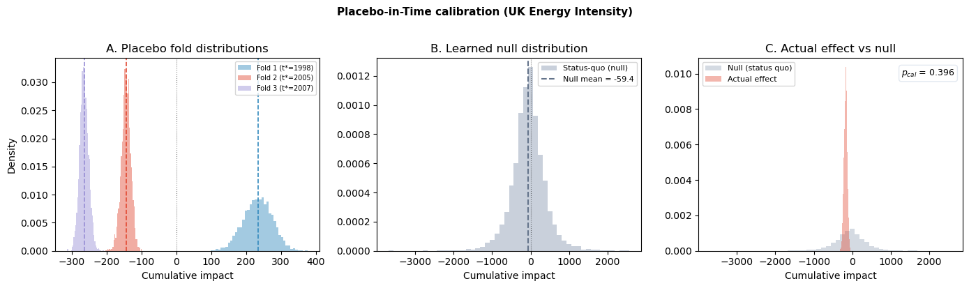
../_images/72653acce5e1ab9e0696b82ef6333608ada898e7de74d3932f5aef5bbf1b09fa.png

This is exactly what we predicted. The effect on total Co2 is weaker, and even when it’s below zero the change it’s perfectly capture by the “usual” mistakes of the model. This support our hypothesis around the redistribution from coal to gas partly cancels out. This is not a failure of the policy; it is consistent with the mechanism. The CPF killed coal, gas absorbed the slack, with other more sustainable sources and the net carbon reduction was smaller than the coal-specific one.

This result also strengthens our causal claim about coal. If the coal Co2 drop were driven by a data error or a recession, we would see the same drop in total Co2. The fact that total Co2 shows a smaller break supports the substitution story.

Did energy demand change?#

The final check. A skeptic’s strongest objection: “Maybe the UK economy crashed in 2013, and the drop in Co2 was just a byproduct of a recession.”

If that were true, the relationship between energy use and economic output would break. We can test this by looking at Energy Intensity (energy_per_gdp) — how much energy it takes to generate one dollar of GDP.

The Carbon Price Floor was designed to clean up the supply side (taxing dirty fuel), not to destroy the demand side (economic output). If the policy worked as intended, the UK economy should have continued generating wealth at its historical rate of energy efficiency. If the energy_per_gdp trend remains perfectly stable through 2013, the recession story collapses.

Note

We switch to a different model here,StateSpaceTimeSeries, to demonstrate that CausalPy’s sensitivity framework works with any estimator. The key assumptions must hold for the specific data and model, but the PlaceboInTime machinery is estimator-agnostic.

sampler_kwargs = {
    "nuts_sampler": "nutpie",
    "nuts_sampler_kwargs": {"backend": "jax", "gradient_backend": "jax"},
    "target_accept": 0.94,
}


def states_space_model():
    """Fresh StateSpaceTimeSeries model (single-use)."""
    return cp.pymc_models.StateSpaceTimeSeries(
        level_order=3,
        seasonal_length=2,
        sample_kwargs=sampler_kwargs,
        mode="FAST_COMPILE",
    )


# Calculate GDP per capita
df_uk_epc = df_uk.dropna(subset=["energy_per_gdp"]).copy()

result_epc = cp.InterruptedTimeSeries(
    data=df_uk_epc[["energy_per_gdp"]],
    treatment_time=treatment_time,
    formula="energy_per_gdp ~ 1",
    model=states_space_model(),
)

                                Model Requirements                                
                                                                                  
  Variable              Shape    Constraints                          Dimensions  
 ──────────────────────────────────────────────────────────────────────────────── 
  initial_level_trend   (3,)                              ('state_level_trend',)  
  sigma_level_trend     (3,)     Positive                 ('shock_level_trend',)  
  params_freq           (1,)                                     ('state_freq',)  
  sigma_freq            ()       Positive                                   None  
  P0                    (5, 5)   Positive semi-definite   ('state', 'state_aux')  
                                                                                  
   These parameters should be assigned priors inside a PyMC model block before    
                    calling the build_statespace_graph method.

Sampler Progress

Total Chains: 4

Active Chains: 0

Finished Chains: 4

Sampling for now

Estimated Time to Completion: now

Draws	Divergences	Step Size	Gradients/Draw
2000	2	0.35	15
2000	3	0.35	15
2000	0	0.36	7
2000	1	0.34	7

Sampling: [obs]

Sampling: [filtered_posterior, filtered_posterior_observed, predicted_posterior, predicted_posterior_observed, smoothed_posterior, smoothed_posterior_observed]

Sampling: [forecast_combined]

fig, axes = result_epc.plot(show=False)
axes[0].set_title("ITS (State-Space) — UK Energy per Capita (Falsification)")
plt.tight_layout()
plt.show()

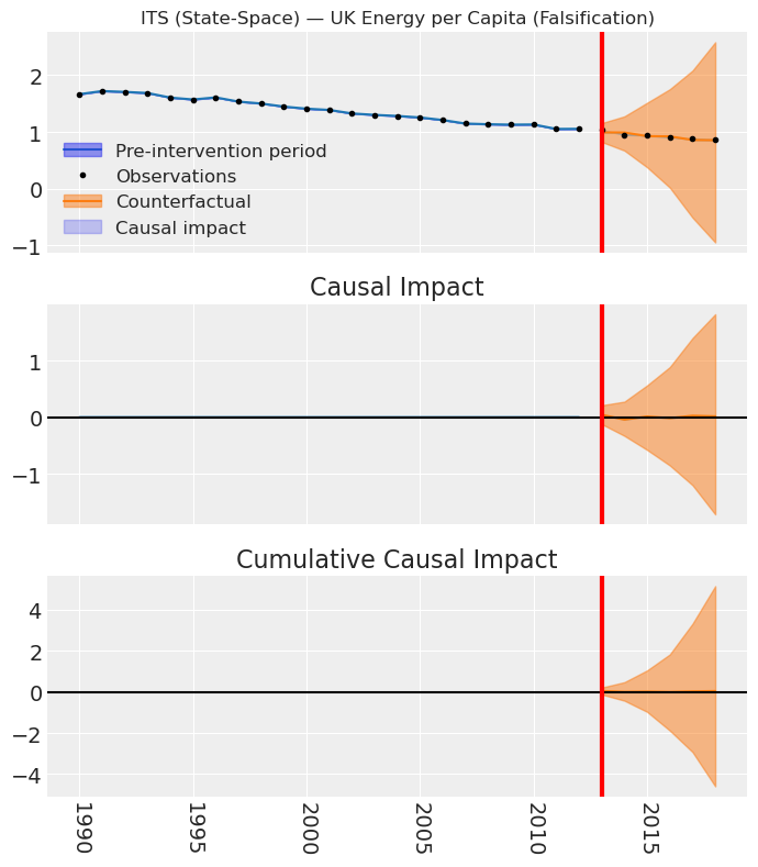
../_images/4d41a8f407747c54c5a4fee58f8155ad2146d540507d0e11db6ae41c2cfae77a.png

Energy per GPD shows no meaningful break at 2013. The actual trajectory hugs the counterfactual. People kept using roughly the same amount of energy — they just stopped getting it from coal.

Assembling the case#

We did not prove that the Carbon Price Floor caused the decline in coal Co2. Proof is not available in observational data. What we did is accumulate four pieces of evidence, each small, each pointing in the same direction:

Step	What we found	What it rules out
Coal Co2 collapsed	Large effect, clearly outside the null	Random fluctuation or model artefact
Gas Co2 rose	Substitution toward gas	General decline in all fuels
Total Co2 effect is weaker	Consistent with redistribution, not elimination	Data error that would affect all Co2 equally
Energy demand stayed flat	Demand unchanged	Recession or demand shock

No single finding is conclusive. But the four together tell a coherent story: the Carbon Price Floor made coal uncompetitive, energy producers switched to gas, coal Co2 collapsed, total Co2 fell modestly, and energy demand was unaffected.